Plotting historical revolutions
Where were revolutions located between 1840 and 1860, based on article titles from Dutch and English newspapers?
The Dutch dataset was constructed querying Delpher on the keyword ‘revolutie’ for the period 1840-1860, with OCR confidence between 80-100 per cent. Since Delpher has no bulk download option, we’ve instead used I-Analyzer (developed by the DH Lab at Utrecht University). This tool allows to query and download Delpher search results for this period. If you want to construct the same dataset from Delpher, you can copy/paste this URL into your browser
The same method has been used to fetch English articles from The Times, for the same period. Only addition is to exclude articles mentioning “industrial”, since “industrial revolution” was also an often used term this period.
To plot the locations mentioned in the article titles several steps are needed: Named Entity Recognition, extracting the locations, geocoding these, and obtaining a map to plot them. Here we’ve used (mainly) R for this, but Python would work as well.
Apart from having R installed, you’ll also need a python executable with spaCy installed, and the corresponding Dutch language model. If you opt for a Google Map you’ll also need a Google API key for its Maps platform. This is free as long as you don’t exceed $200 in API calls a month (which usually does’t happen).
First we load the required libraries and the Delpher dataset.
library(data.table)
library(spacyr)
library(maps)
library(rasterVis)
library(raster)
library(ggmap)
library(ggplot2)
library(ggpubr)

revol <- fread("C:\\Users\\Schal107\\Documents\\UBU\\Team DH\\Delpher\\dutchnewspapers-public_query=revolutie_date=1840-01-01 1860-12-31_ocr=80 100_sort=date,desc.csv")
setDT(revol)
Let’s keep only the variables we want to continue to work with. And inspect the first rows of this subset. You’ll already notice the mentioning of “FRANKRIJK” (France) and “WEENEN” (Vienna) here.
x <- revol[,c("date", "article_title", "url")]
x[5851:5858]
## date article_title
## 1: 1848-10-13 REVOLUTIE IN WEENEN OP DEN 6 EN 7 OCTOBER.
## 2: 1848-10-13 ZWITSERLAND. BERN 8 Oct.
## 3: 1848-10-13 Brussel , 11 October.
## 4: 1848-10-12 FRANKRIJK. PARIJS, den 8sten October.
## 5: 1848-10-12 Een blik op FrankrijKs consti- tuerende vergadering.
## 6: 1848-10-10 LONDEN. 7 October ('savonds).
## 7: 1848-10-10 FRANKRIJK. PARIJS, 3 October.
## 8: 1848-10-10 DUITSCHLAND.
## url
## 1: http://resolver.kb.nl/resolve?urn=ddd:010772343:mpeg21:a0051
## 2: http://resolver.kb.nl/resolve?urn=ddd:010779162:mpeg21:a0002
## 3: http://resolver.kb.nl/resolve?urn=ddd:010067138:mpeg21:a0009
## 4: http://resolver.kb.nl/resolve?urn=ddd:010174429:mpeg21:a0001
## 5: http://resolver.kb.nl/resolve?urn=ddd:010151491:mpeg21:a0001
## 6: http://resolver.kb.nl/resolve?urn=ddd:010519531:mpeg21:a0007
## 7: http://resolver.kb.nl/resolve?urn=ddd:010772342:mpeg21:a0017
## 8: http://resolver.kb.nl/resolve?urn=ddd:010929387:mpeg21:a0008Not required for now, but below demonstrates how to extract years from the date variable.
x$date <- as.Date(x$date)
x[, year := as.numeric(substr(x$date, 1,4))]
setDT(x)
x[, .N, list(year)][order(-year)][1:10]
## year N
## 1: 1860 1006
## 2: 1859 806
## 3: 1858 290
## 4: 1857 321
## 5: 1856 471
## 6: 1855 217
## 7: 1854 317
## 8: 1853 328
## 9: 1852 290
## 10: 1851 404For better Named Entity Recognition we will change the article_title variable to lower case strings. SpaCy has the tendency to recognize uppercase strings as corporations.
x$article_title <- tolower(x$article_title)Now we need to call in action the Dutch language model from spaCy to perform NER. If you want to replicate this analysis, you need to have this installed on your local machine. Read the website for installation instructions.
spacy_initialize(model = "nl_core_news_sm")Below we parse the article_title to SpaCy and perform NER. You’ll see that it has recognized at least some locations.
parsedtxt <- spacy_parse(x$article_title, lemma = FALSE, entity = TRUE, nounphrase = TRUE)

locations <- entity_extract(parsedtxt)

setDT(locations)
top100 <- locations[entity_type == "GPE", .N, list(entity) ][order(-N)]

head(top100)
## entity N
## 1: frankrijk 1013
## 2: parijs 883
## 3: amsterdam 697
## 4: brussel 107
## 5: utrecht 106
## 6: londen 97Before we can plot them on a map, we need to add coordinates to the placenames. We’ll use the Google Maps API for that. Notice that you will need your own key to do so. You can register for a free API key at Google.
google_key <- fread("C:\\Users\\Schal107\\Documents\\UBU\\Team DH\\Delpher\\google_key.txt")
register_google(key = paste0(google_key$key))

coordinates <- geocode(top100$entity)

head(coordinates)
## # A tibble: 6 x 2
## lon lat
## <dbl> <dbl>
## 1 2.21 46.2
## 2 2.35 48.9
## 3 4.90 52.4
## 4 4.36 50.8
## 5 5.12 52.1
## 6 -0.128 51.5After the geocoding we merge the retrieved coordinates with the placenames.
coordinates_delpher <- cbind(top100, coordinates)
head(coordinates_delpher)
## entity N lon lat
## 1: frankrijk 1013 2.2137490 46.22764
## 2: parijs 883 2.3522219 48.85661
## 3: amsterdam 697 4.9041389 52.36757
## 4: brussel 107 4.3571696 50.84764
## 5: utrecht 106 5.1214201 52.09074
## 6: londen 97 -0.1275862 51.50722Now we’ll do the same for articles from The Times
You can reconstruct the Times dataset using this I-analyzer URL.
times <- fread("C:\\Users\\Schal107\\Documents\\UBU\\Team DH\\Delpher\\times_query=revolution_-_industrial_date=1840-01-01 1860-12-31_ocr=80 100.csv")
colnames(times)
## [1] "edition" "issue" "volume" "date-pub" "content" "title" "ocr"
## [8] "id"Now we’ll perform Named Entity Recognition and geocoding on the English titles.
spacy_initialize(model = "en_core_web_sm")## NULLparsedtxt2 <- spacy_parse(times$title, lemma = FALSE, entity = TRUE, nounphrase = TRUE)
locations2 <- entity_extract(parsedtxt2)
setDT(locations2)
times_locations <- locations2[entity_type == "GPE", .N, list(entity) ][order(-N)]
head(times_locations)## entity N
## 1: Friday 147
## 2: Wednesday 98
## 3: Ireland 87
## 4: Thursday 47
## 5: India 40
## 6: Madrid 29coordinates_times <- geocode(times_locations$entity)
coordinates_times <- cbind(times_locations, coordinates_times)
head(coordinates_times)## entity N lon lat
## 1: Friday 147 NA NA
## 2: Wednesday 98 NA NA
## 3: Ireland 87 -7.692054 53.14237
## 4: Thursday 47 NA NA
## 5: India 40 78.962880 20.59368
## 6: Madrid 29 -3.703790 40.41678We now have two datasets with placenames and coordinates together with the number of times these places appeared in newspaper titles. Before plotting, we remove locations without coordinates.
coordinates_times[, dataset := "times",]
coordinates_delpher[, dataset := "delpher"]
setnames(coordinates_times, "N", "n_times")
setnames(coordinates_delpher, "N", "n_delpher")

setnames(coordinates_times, "entity", "entity_times")
setnames(coordinates_delpher, "entity", "entity_delpher")

coordinates_times <- coordinates_times[!is.na(lon),]
coordinates_delpher <- coordinates_delpher[!is.na(lon),]
Final: plot coordinates from Delpher and Times on a map
Now we’ll need a map! You can use the standard Google Map and define
a centre using latitute and longitude. However, for historical data I
like to remove roads and names from the map. You can do that by making
your own map at Google
Mapstyle. With the same API key as you’ve use for the geocoding, you
can export the URL of your map of choice, and paste it below in the
function get_googlemap. For some reason, though, you first
need to extract the lat and long from this URL, and the zoom level (see
below). Then you paste the remaining URL from the first mention of
‘&maptype’ behind path = (don’t forget to include it in
quotes). Then it should work!
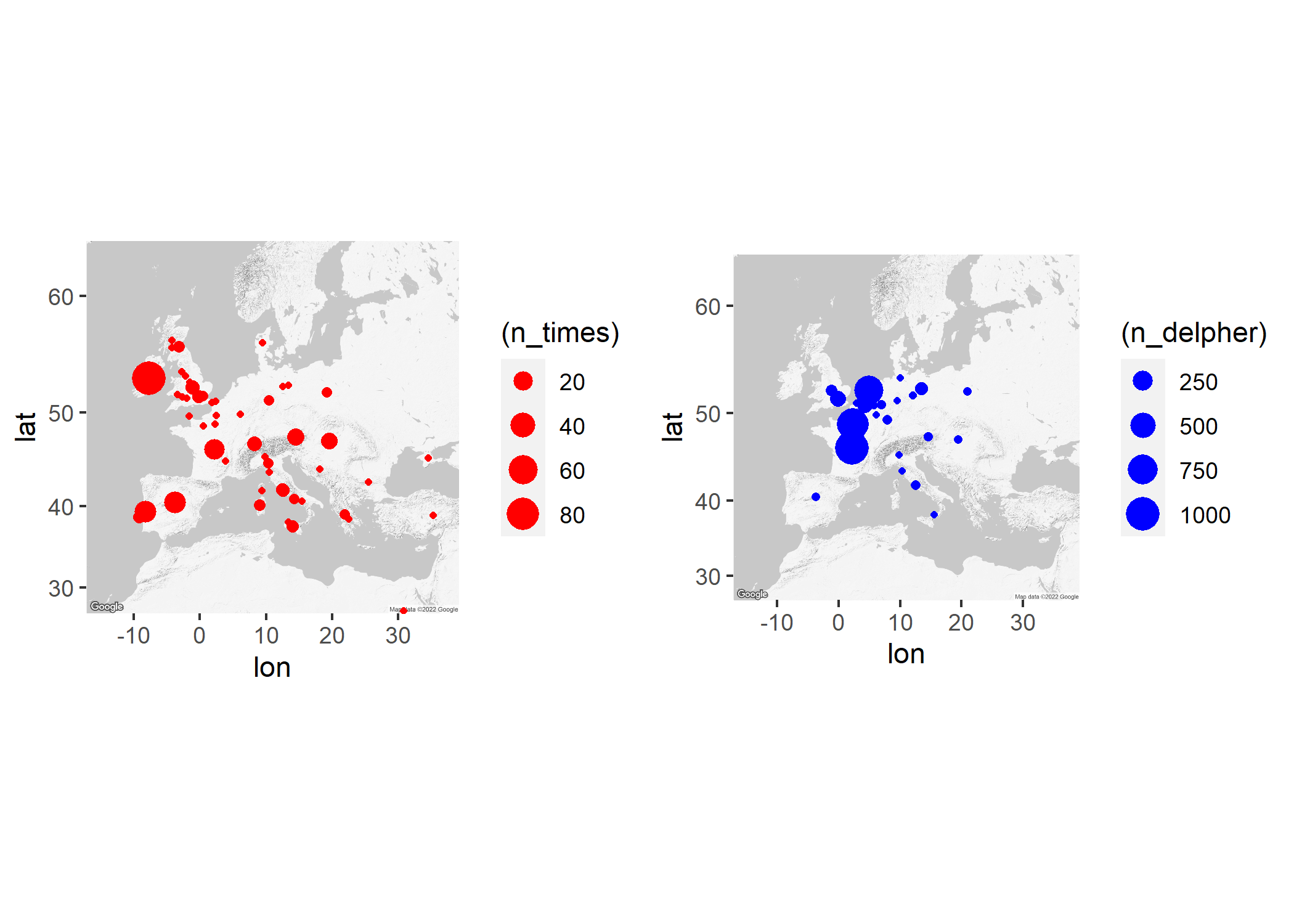
europe5 <- get_googlemap(center=c(lon=10.95931966568949, lat=48.561877580811775), zoom = 4, path = "&maptype=roadmap&style=element:geometry%7Ccolor:0xf5f5f5&style=element:labels%7Cvisibility:off&style=element:labels.icon%7Cvisibility:off&style=element:labels.text.fill%7Ccolor:0x616161&style=element:labels.text.stroke%7Ccolor:0xf5f5f5&style=feature:administrative.land_parcel%7Cvisibility:off&style=feature:administrative.land_parcel%7Celement:labels.text.fill%7Ccolor:0xbdbdbd&style=feature:administrative.neighborhood%7Cvisibility:off&style=feature:landscape.natural.terrain%7Ccolor:0xffffff%7Cvisibility:on%7Cweight:4&style=feature:landscape.natural.terrain%7Celement:geometry.fill%7Cvisibility:on%7Cweight:4&style=feature:landscape.natural.terrain%7Celement:geometry.stroke%7Cvisibility:on&style=feature:poi%7Celement:geometry%7Ccolor:0xeeeeee&style=feature:poi%7Celement:labels.text.fill%7Ccolor:0x757575&style=feature:poi.park%7Celement:geometry%7Ccolor:0xe5e5e5&style=feature:poi.park%7Celement:labels.text.fill%7Ccolor:0x9e9e9e&style=feature:road%7Cvisibility:off&style=feature:road%7Celement:geometry%7Ccolor:0xffffff&style=feature:road.arterial%7Celement:labels.text.fill%7Ccolor:0x757575&style=feature:road.highway%7Celement:geometry%7Ccolor:0xdadada&style=feature:road.highway%7Celement:labels.text.fill%7Ccolor:0x616161&style=feature:road.local%7Celement:labels.text.fill%7Ccolor:0x9e9e9e&style=feature:transit.line%7Celement:geometry%7Ccolor:0xe5e5e5&style=feature:transit.station%7Celement:geometry%7Ccolor:0xeeeeee&style=feature:water%7Celement:geometry%7Ccolor:0xc9c9c9&style=feature:water%7Celement:labels.text.fill%7Ccolor:0x9e9e9e&size=480x360")Now that we have our map loaded, we parse it to ggmap. Then we can add our data to it. The size of the dots corresponds to the number of times the geocoded placename is mentioned in our article titles. You’ll see that Paris and France are dominant, but also that we spot some unexpected places in Italy and even Eastern Europe.
p <- ggmap(europe5)
times <- p + geom_point(data = coordinates_times, aes(x=lon, y=lat, size=(n_times)), shape=16, color = "red")
invisible(ggplot_build(times))
ggsave("times_map.png")

p <- ggmap(europe5)
delpher <- p + geom_point(data = coordinates_delpher, aes(x=lon, y=lat, size=(n_delpher)), shape=16, color = "blue")
invisible(ggplot_build(delpher))
ggsave("delpher_map.png")

invisible(ggarrange(times, delpher))
ggsave("all_map.png")
And here we have our results!
(The geocoded datasets are available at the Github repository.)
Colophon
This notebook was created by Utrecht University Library, Digital Humanities Support
For questions and suggestions please email Ruben Schalk
Last updated on 29 augustus, 2022